R Training | Day 2
Good morning Jedis!

Schedule
- Review Day 1
- The
ggplot()sandwich - Explore your
data frame - Arrange and filter data
- Guess Who! - The Star Wars edition
Review
- We kicked off with a tour of RStudio.
- Then learned to:
- Store values
- Name objects
- Remove objects
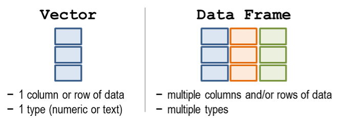
- Made lists with
c("item 1", "item 2", "item 3") - Combined multiple lists into a tidy table
- R calls these
data frames
- R calls these
- Installed NEW packages


- Read data from online using
read_csv() - Used the
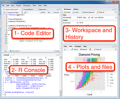
ggplot()function to make our first plot
Example workflow
Here’s an example air monitoring project from start to finish.
EXAMPLE - Ozone data project
Imagine we just received 3 years worth of ozone monitoring data to summarize. Fun! Below is an example workflow we might follow using R.
0. Start a new project
Let’s be creative and name our project: "2019_Ozone"
1. Read the data
library(readr)

# Read a file from the web
air_data <- read_csv("https://itep-r.netlify.com/data/OZONE_samples_demo.csv")| SITE | Date | OZONE | TEMP_F |
|---|---|---|---|
| 27-137-7554 | 2018-05-06 | 6 | 45.8 |
| 27-137-7001 | 2016-08-24 | 13 | 70.4 |
| 27-137-7001 | 2016-08-05 | 11 | 77.0 |
| 27-137-7554 | 2018-07-14 | 17 | 58.4 |
| 27-137-7554 | 2017-09-05 | 11 | 59.6 |
2. Clean the names
library(janitor)

# Capital letters and spaces make things more difficult
# Let's clean them out
air_data <- clean_names(air_data)
3. Plot the data
library(ggplot2)

ggplot(air_data, aes(x = temp_f, y = ozone)) +
    geom_point(alpha = 0.2) +
    geom_smooth(method = "lm")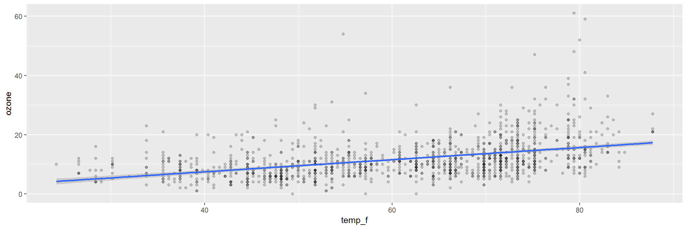
4. Clean the data
library(dplyr)

# Drop values out of range
air_data <- air_data %>% filter(ozone > 0, temp_f < 199)

# Convert all samples to PPB
air_data <- air_data %>%
            mutate(OZONE = ifelse(units == "PPM", ozone * 1000,
                                  ozone))
5. View the data closer
ggplot(air_data, aes(x = temp_f, y = ozone)) +
    geom_point(alpha = 0.2, size = 3) +
    geom_smooth(method = "lm") +
    facet_wrap(~site) +
    labs(title = "Ozone increases with temperature",
         subtitle = "Observations from 2015-2017")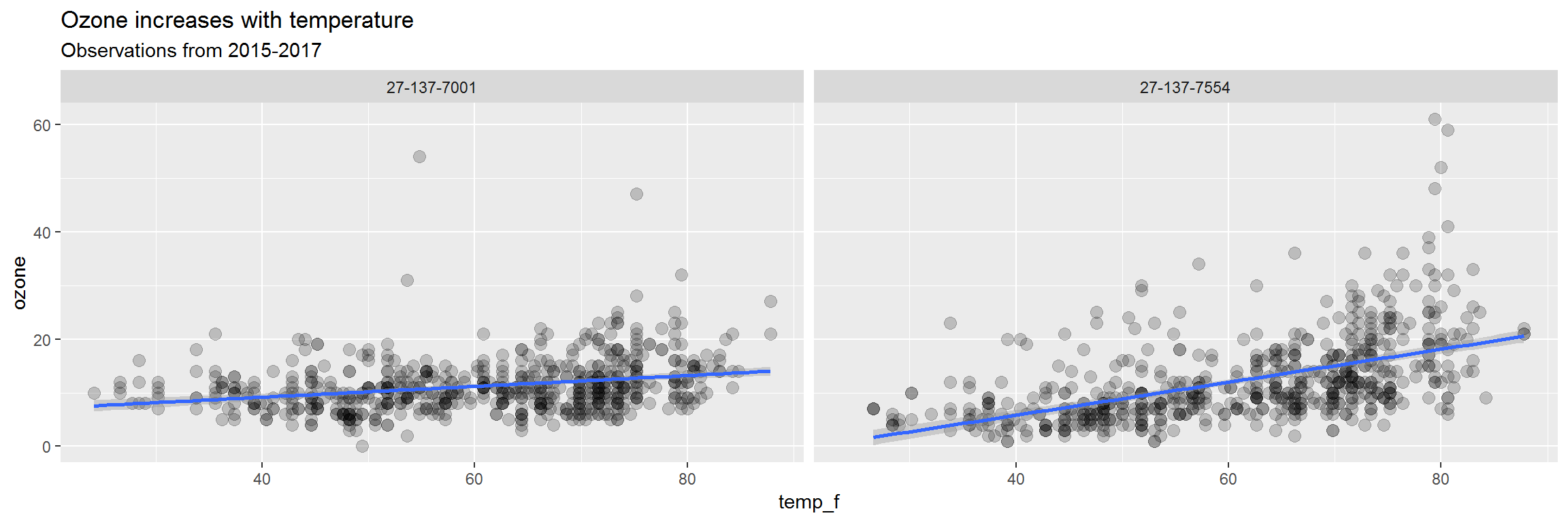
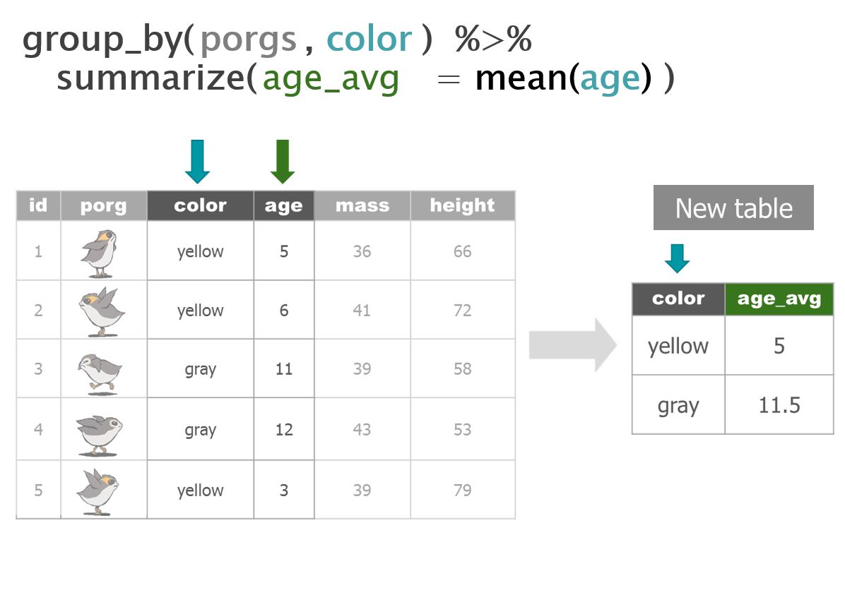
6. Summarize the data
air_data <- air_data %>%
            group_by(site, year) %>%
            summarize(avg_ozone = mean(ozone) %>% round(2),
avg_temp = mean(temp_f) %>% round(2))| site | year | avg_ozone | avg_temp |
|---|---|---|---|
| 27-137-7001 | 2016 | 11.01 | 60.74 |
| 27-137-7001 | 2017 | 11.26 | 60.66 |
| 27-137-7001 | 2018 | 11.54 | 60.59 |
| 27-137-7554 | 2016 | 12.23 | 61.23 |
| 27-137-7554 | 2017 | 11.81 | 60.98 |
| 27-137-7554 | 2018 | 12.87 | 61.02 |
7. Save the results
Save the final data table
air_data %>% write_csv("results/2015-17_ozone_summary.csv")Save the site plot to PDF
ggsave("results/2015-2017 - Ozone vs Temp.pdf")8. Share with friends
Having an exact record of what you did can be great documentation for yourself and others. It’s also handy when you want to repeat the same analysis on new data. Then you only need to copy the script, update the read data line, and push run to get a whole new set of fancy charts.
Back to Jakku!

A new day
Let’s start fresh with a new R script.
OPEN a new R script
- File > New File > R Script
- Click the floppy disk save icon
- Give it a name:
day2.Rwill work well
Load the readr package from our library
library(readr)Read the scrap data from the web
# Read in scrap data and set name to "scrap"
scrap <- read_csv("https://itep-r.netlify.com/data/starwars_scrap_jakku.csv")
Plot the scrap data
Last time we made a column plot showing the amount of scrap coming from each origin city.
library(ggplot2)

ggplot(scrap, aes(y = amount, x = origin)) +
  geom_col() +
labs(title = "Which origin sold the most scrap?") 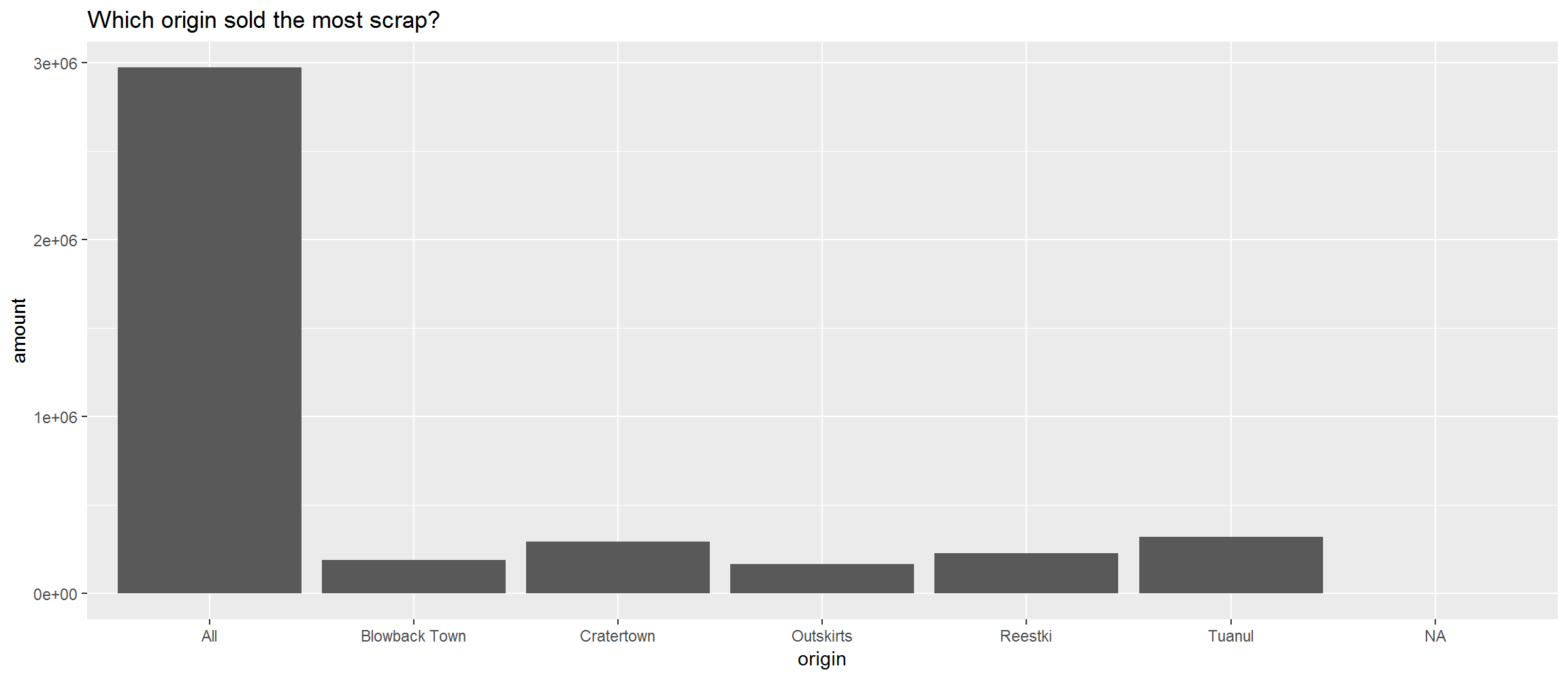
Let’s break this down into its main ingredients and get to know ggplot().
1 | Plots with ggplot2
Plot the data, Plot the data, Plot the data
The ggplot() sandwich
A ggplot has 3 ingredients.
1. The base plot
library(ggplot2)ggplot(scrap)
we load the package
library (ggplot2), but the function to make a plot isggplot(scrap).
2. The the X, Y aesthetics
The aesthetics assign the components from the data that you want to use in the chart. These also determine the dimensions of the plot.
ggplot(scrap, aes(x = origin, y = amount)) 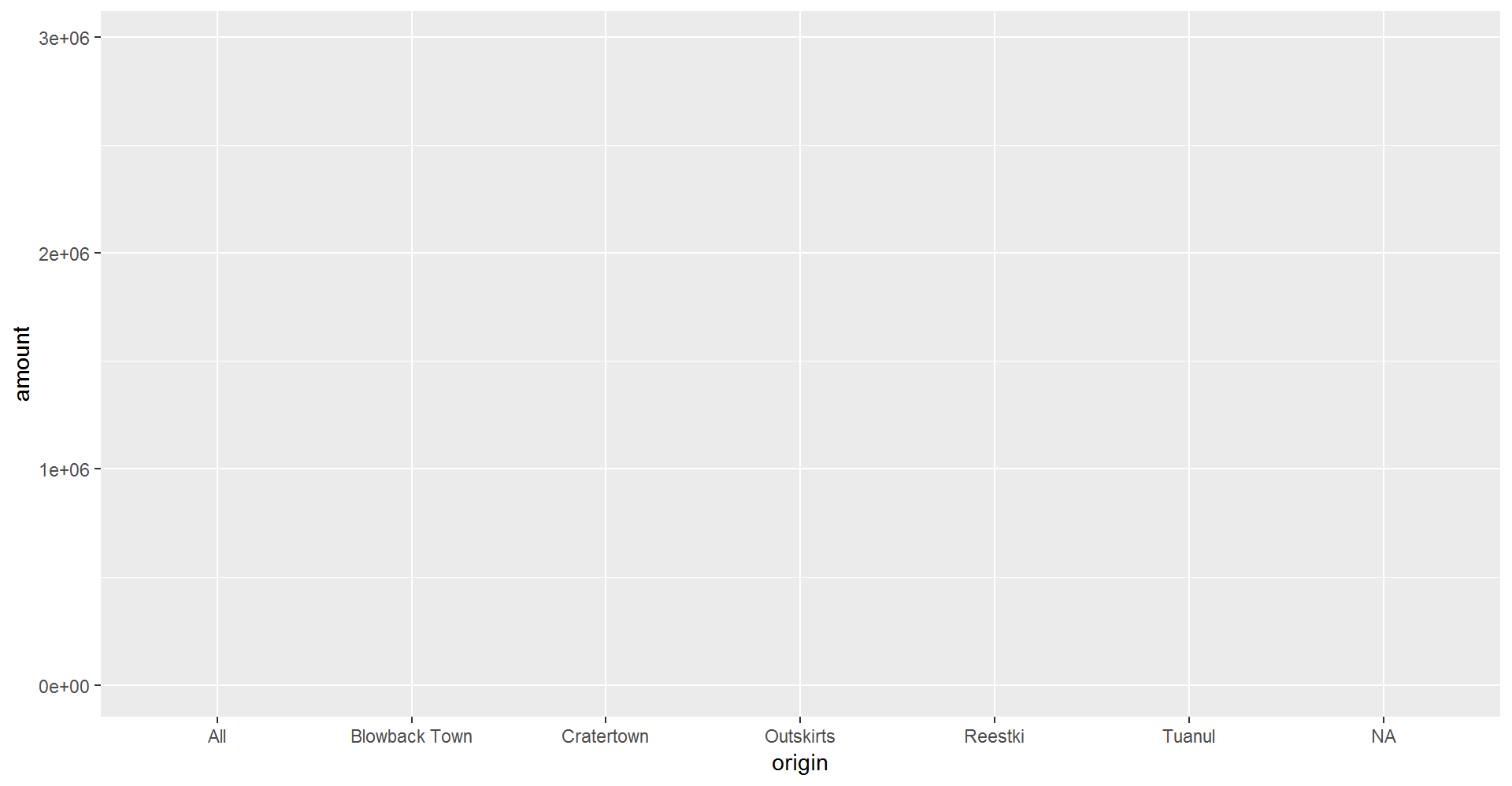
3. The layers or geometries
ggplot(scrap, aes(x = origin, y = amount)) + geom_col()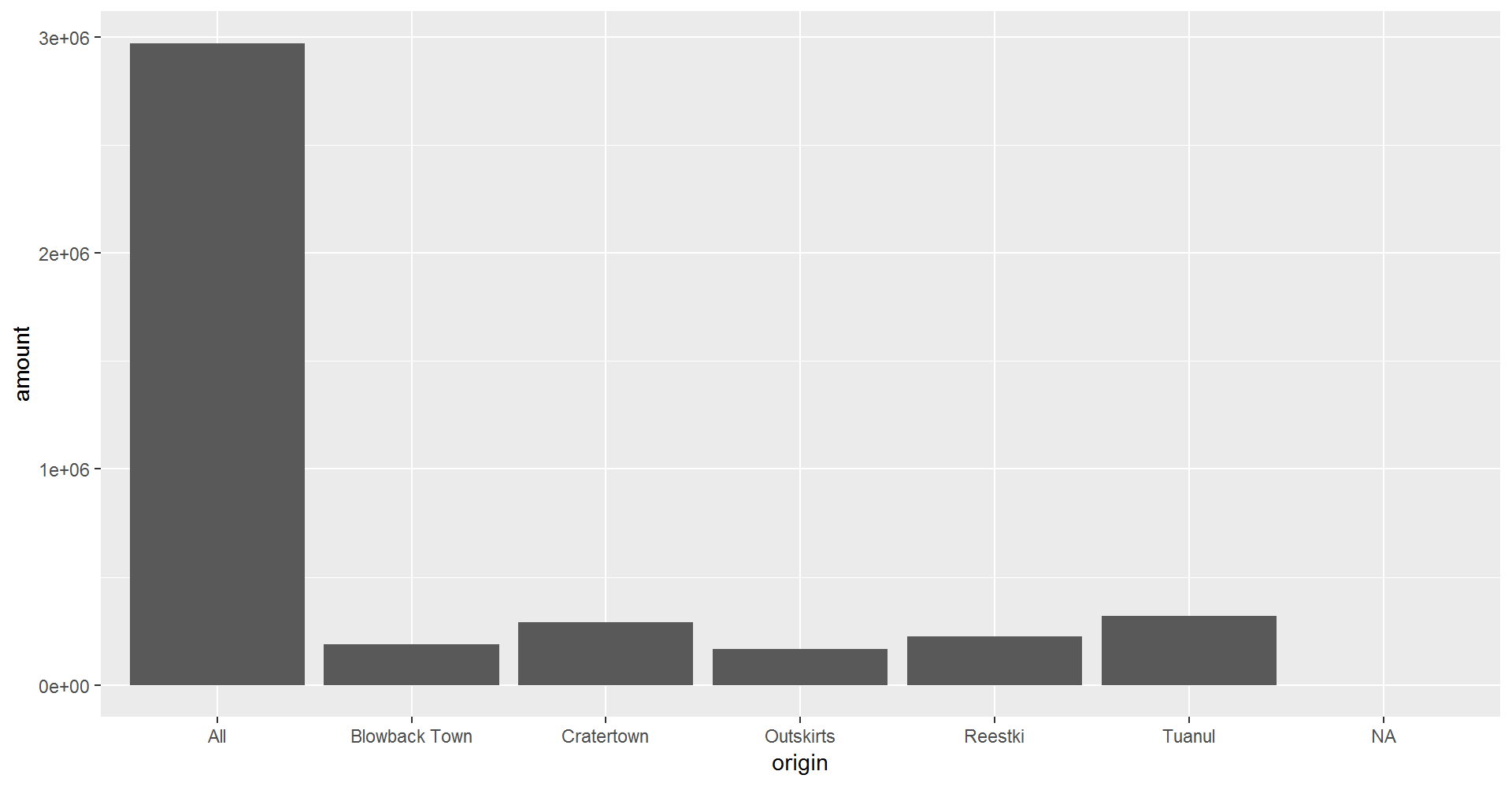
Colors
Now let’s change the fill color to match the origin.
ggplot(scrap, aes(x = origin, y = amount, fill = origin)) +
geom_col() 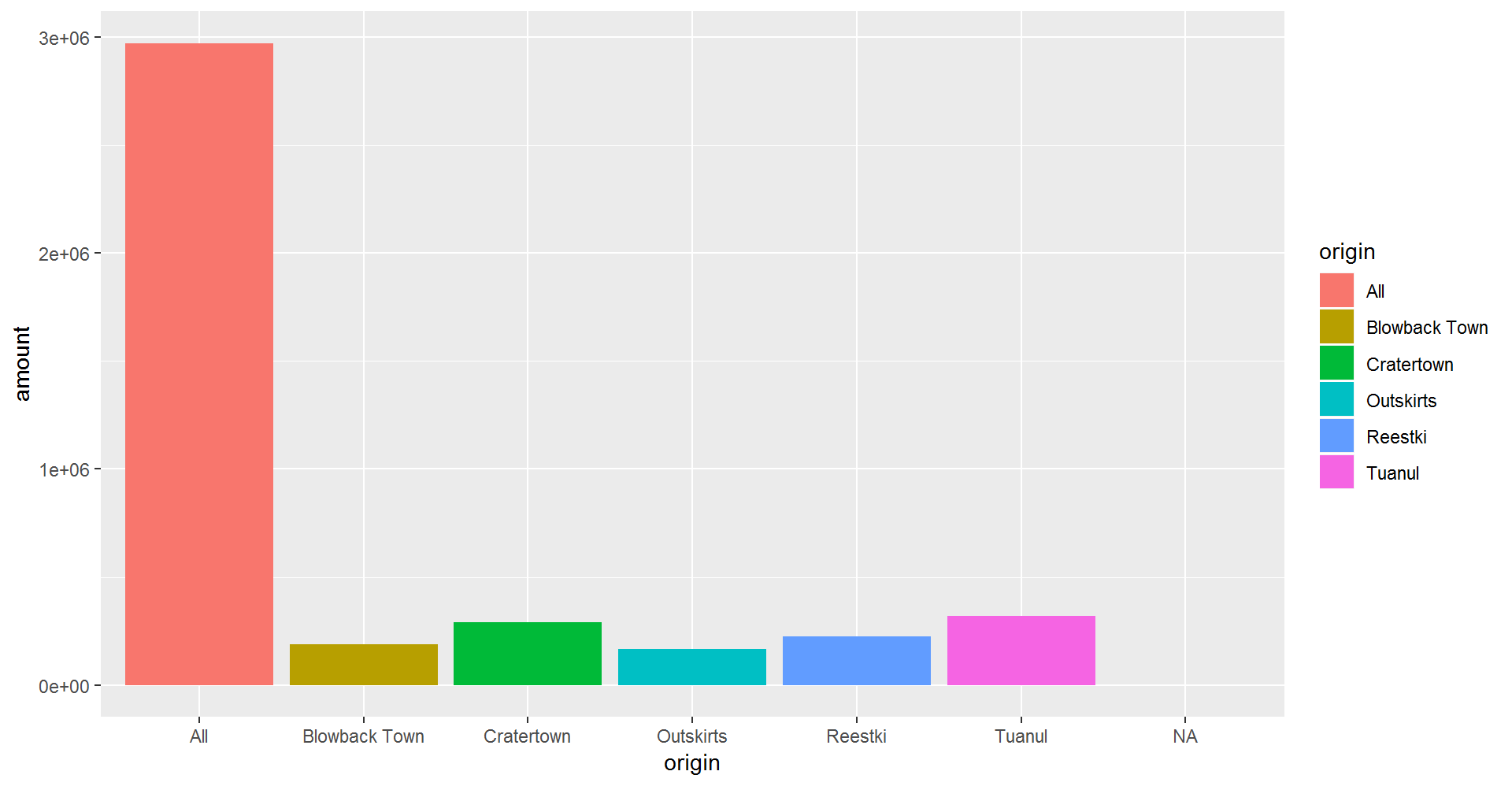
EXERCISE
Try making a column plot showing the total amount of scrap for each destination or for each item.
ggplot(scrap, aes(x = destination, y = amount )) + geom_col()It’s officially time to solve our “All” city issue.
Data exploration
2 | dplyr

The dplyr package is our go-to tool for exploring, re-arranging, and summarizing data. Use install.packages("dplyr") to add dplyr to your library.
Functions to get to know your data.
| Function | Information |
|---|---|
names(scrap) |
column names |
nrow(...) |
number of rows |
ncol(...) |
number of columns |
summary(...) |
summary of all column values (ex. max, mean, median) |
glimpse(...) |
column names + a glimpse of first values (requires dplyr package) |
3 | glimpse() the columns
Use the glimpse() function to find out what type and how much data you have.
Use the summary() function to get a quick report on your numeric data.
Let’s give these a whirl.
library(dplyr)

# View the first few values & the type of data each column contains
glimpse(scrap)
## Observations: 1,132
## Variables: 7
## $ receipt_date <chr> "4/1/2013", "4/2/2013", "4/3/2013", "4/4/2013"...
## $ item <chr> "Flight recorder", "Proximity sensor", "Vitus-...
## $ origin <chr> "Outskirts", "Outskirts", "Reestki", "Tuanul",...
## $ destination <chr> "Niima Outpost", "Raiders", "Raiders", "Raider...
## $ amount <dbl> 887, 7081, 4901, 707, 107, 32109, 862, 13944, ...
## $ units <chr> "Tons", "Tons", "Tons", "Tons", "Tons", "Tons"...
## $ price_per_pound <dbl> 590.93, 1229.03, 225.54, 145.27, 188.28, 1229....# Use the summary function to get a quick of idea of means and maxima for your numeric data
summary(scrap)## receipt_date item origin
## Length:1132 Length:1132 Length:1132
## Class :character Class :character Class :character
## Mode :character Mode :character Mode :character
##
##
##
##
## destination amount units
## Length:1132 Min. : 65 Length:1132
## Class :character 1st Qu.: 1544 Class :character
## Mode :character Median : 4099 Mode :character
## Mean : 18751
## 3rd Qu.: 7475
## Max. :2971601
## NA's :910
## price_per_pound
## Min. : 145.3
## 1st Qu.: 259.6
## Median : 790.7
## Mean : 3811.7
## 3rd Qu.: 1496.7
## Max. :579215.3
## NA's :910# Try the rest on your own - be BRAVE!
nrow()
ncol()
names()More dplyr
dplyr is our go-to package for most analysis tasks. With the six functions below you can accomplish just about anything you’d want to do with data.
Your new analysis toolbox
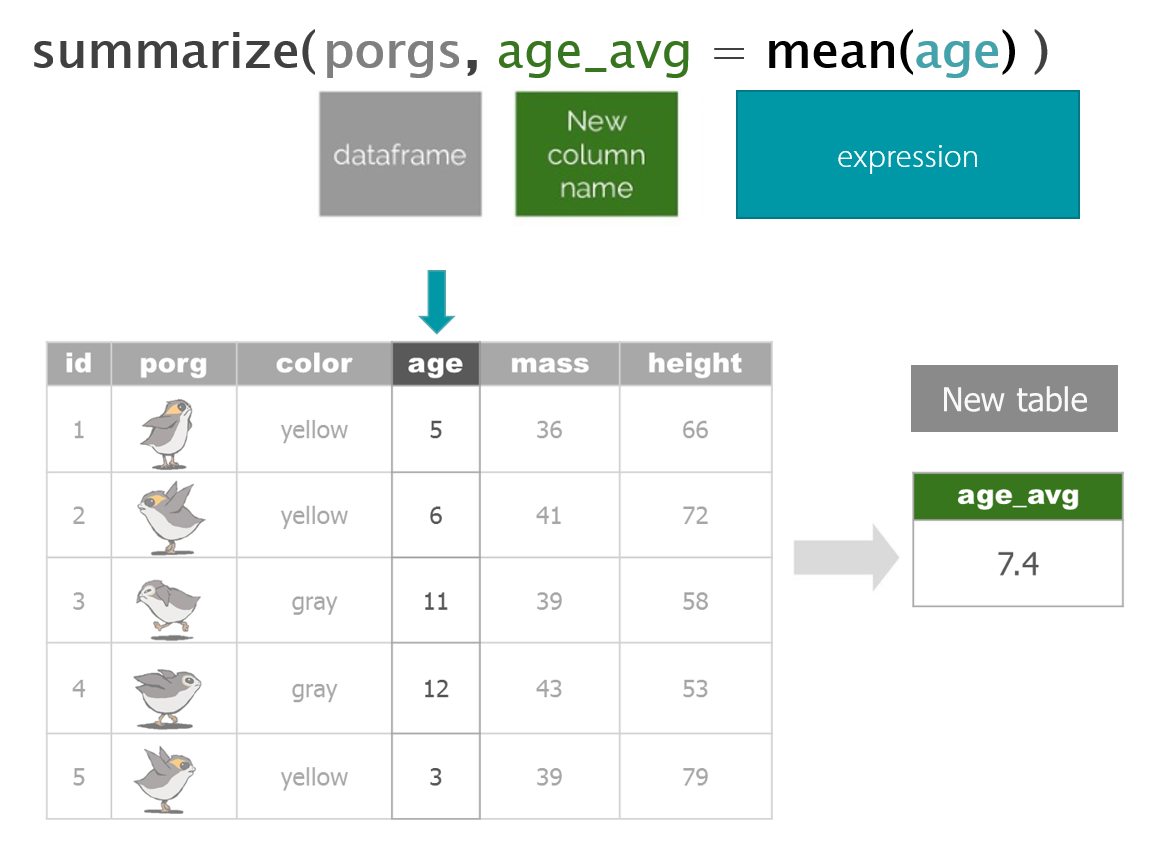
Function Job select()Select individual columns to drop or keep arrange()Sort a table top-to-bottom based on the values of a column filter()Keep only a subset of rows depending on the values of a column mutate()Add new columns or update existing columns summarize()Calculate a single summary for an entire table group_by()Sort data into groups based on the values of a column
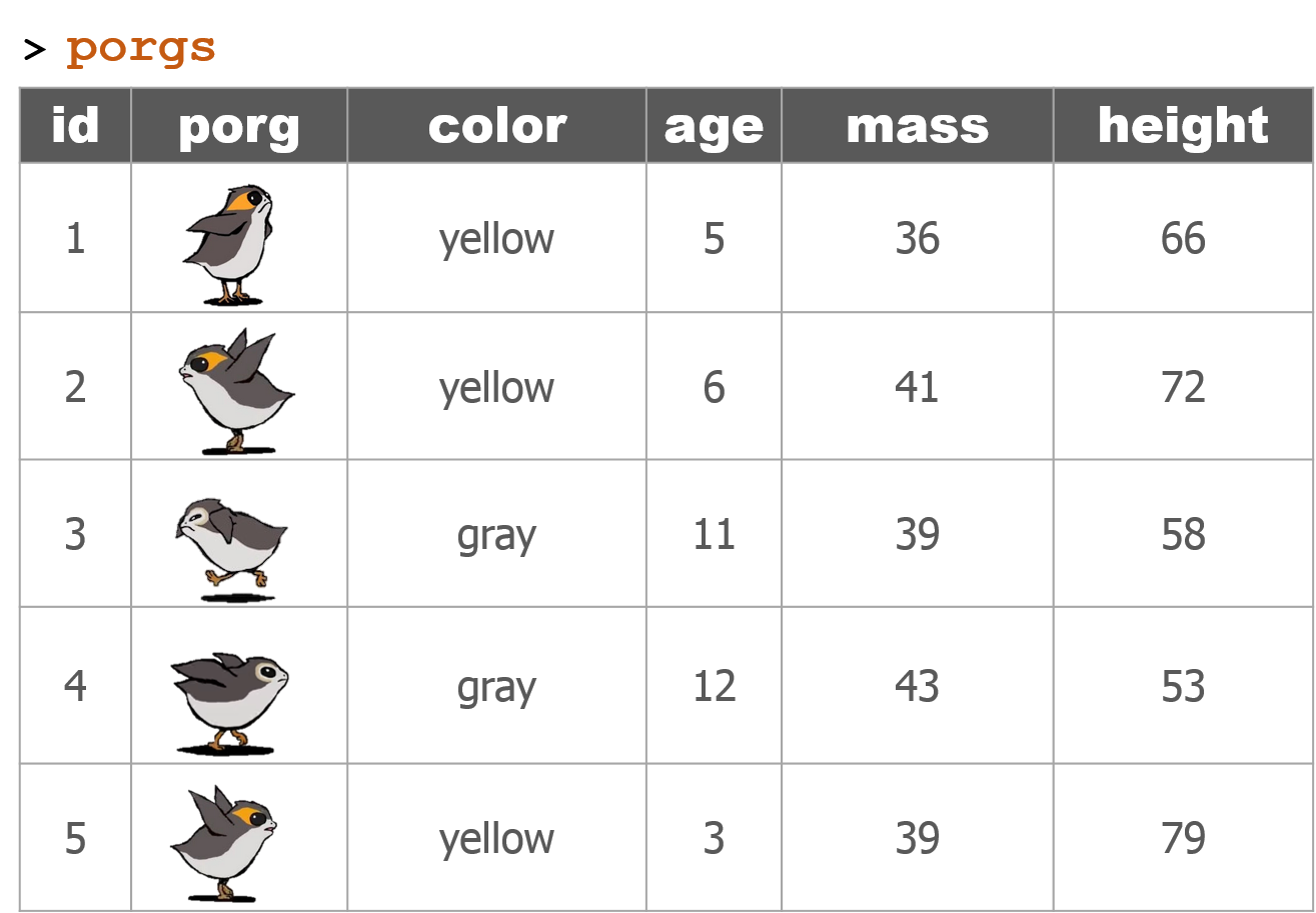
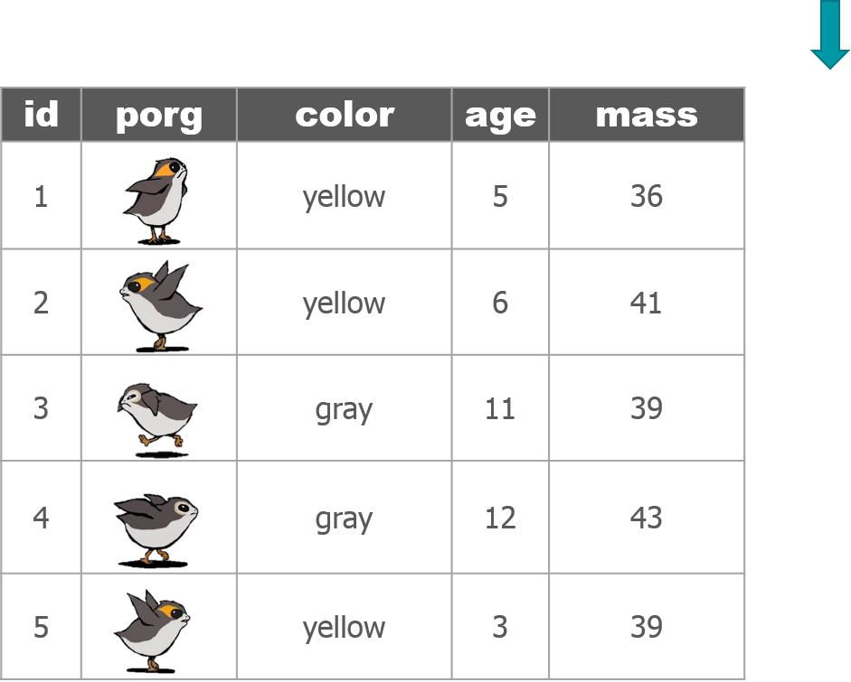
4 | Porg tables
A poggle of porgs has volunteered to help us demo the dplyr functions.
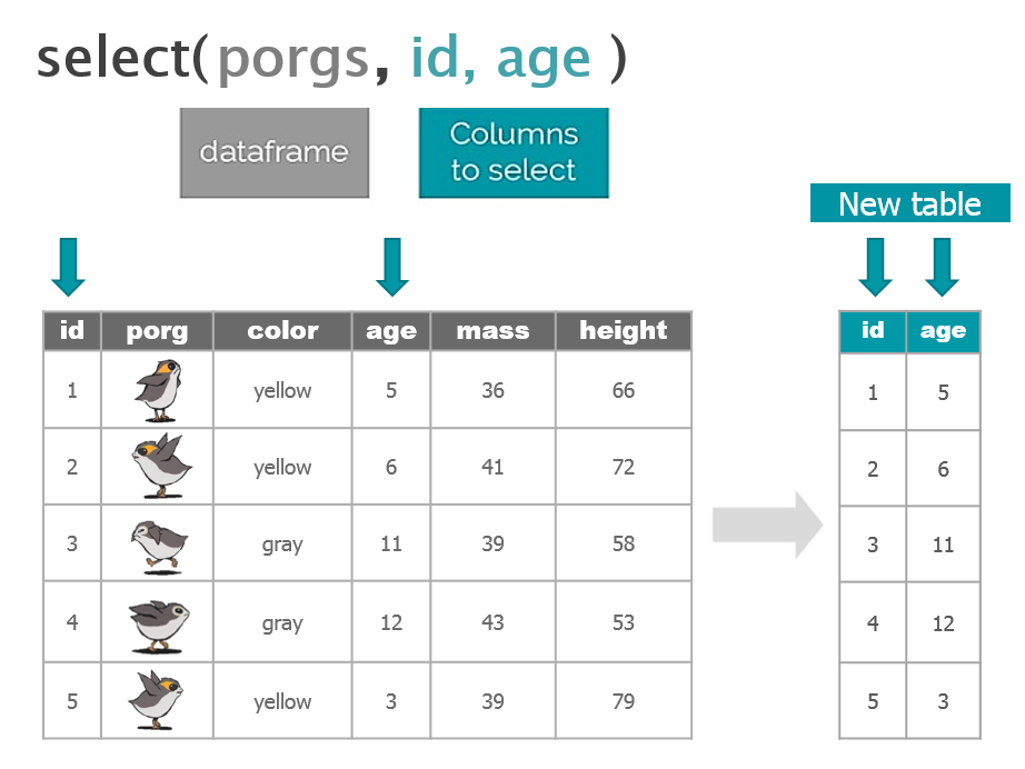


5 | select()
Use the select() function to:
- Drop a column you no longer need
- Pull-out a few columns to create a new table
- Rearrange or change the order of columns
Drop columns with a minus sign: -column_name
library(dplyr)
library(readr)

scrap <- read_csv("https://itep-r.netlify.com/data/starwars_scrap_jakku.csv")

# Drop the destination column
select(scrap, -destination)
## # A tibble: 1,132 x 6
## receipt_date item origin amount units price_per_pound
## <chr> <chr> <chr> <dbl> <chr> <dbl>
## 1 4/1/2013 Flight recorder Outskir~ 887 Tons 591.
## 2 4/2/2013 Proximity sensor Outskir~ 7081 Tons 1229.
## 3 4/3/2013 Vitus-Series Attitud~ Reestki 4901 Tons 226.
## 4 4/4/2013 Aural sensor Tuanul 707 Tons 145.
## 5 4/5/2013 Electromagnetic disc~ Tuanul 107 Tons 188.
## 6 4/6/2013 Proximity sensor Tuanul 32109 Tons 1229.
## 7 4/7/2013 Hyperdrive motivator Tuanul 862 Tons 1485.
## 8 4/8/2013 Landing jet Reestki 13944 Tons 1497.
## 9 4/9/2013 Electromagnetic disc~ Cratert~ 7788 Tons 188.
## 10 4/10/2013 Sublight engine Outskir~ 10642 Tons 7211.
## # ... with 1,122 more rowsKeep only three columns
# Keep the item, amount and price_per_pound columns
select(scrap, c(item, amount, price_per_pound))
## # A tibble: 1,132 x 3
## item amount price_per_pound
## <chr> <dbl> <dbl>
## 1 Flight recorder 887 591.
## 2 Proximity sensor 7081 1229.
## 3 Vitus-Series Attitude Thrusters 4901 226.
## 4 Aural sensor 707 145.
## 5 Electromagnetic discharge filter 107 188.
## 6 Proximity sensor 32109 1229.
## 7 Hyperdrive motivator 862 1485.
## 8 Landing jet 13944 1497.
## 9 Electromagnetic discharge filter 7788 188.
## 10 Sublight engine 10642 7211.
## # ... with 1,122 more rowseverything()
select() also works to change the order of columns. The code below puts the item column first and then moves the units and amount columns directly after item. We then keep everything() else the same.
# Make the `item`, `units`, and `amount` columns the first three columns
# Leave `everything()` else in the same order
select(scrap, item, units, amount, everything())
## # A tibble: 1,132 x 7
## item units amount receipt_date origin destination price_per_pound
## <chr> <chr> <dbl> <chr> <chr> <chr> <dbl>
## 1 Flight re~ Tons 887 4/1/2013 Outski~ Niima Outp~ 591.
## 2 Proximity~ Tons 7081 4/2/2013 Outski~ Raiders 1229.
## 3 Vitus-Ser~ Tons 4901 4/3/2013 Reestki Raiders 226.
## 4 Aural sen~ Tons 707 4/4/2013 Tuanul Raiders 145.
## 5 Electroma~ Tons 107 4/5/2013 Tuanul Niima Outp~ 188.
## 6 Proximity~ Tons 32109 4/6/2013 Tuanul Trade cara~ 1229.
## 7 Hyperdriv~ Tons 862 4/7/2013 Tuanul Trade cara~ 1485.
## 8 Landing j~ Tons 13944 4/8/2013 Reestki Niima Outp~ 1497.
## 9 Electroma~ Tons 7788 4/9/2013 Crater~ Raiders 188.
## 10 Sublight ~ Tons 10642 4/10/2013 Outski~ Niima Outp~ 7211.
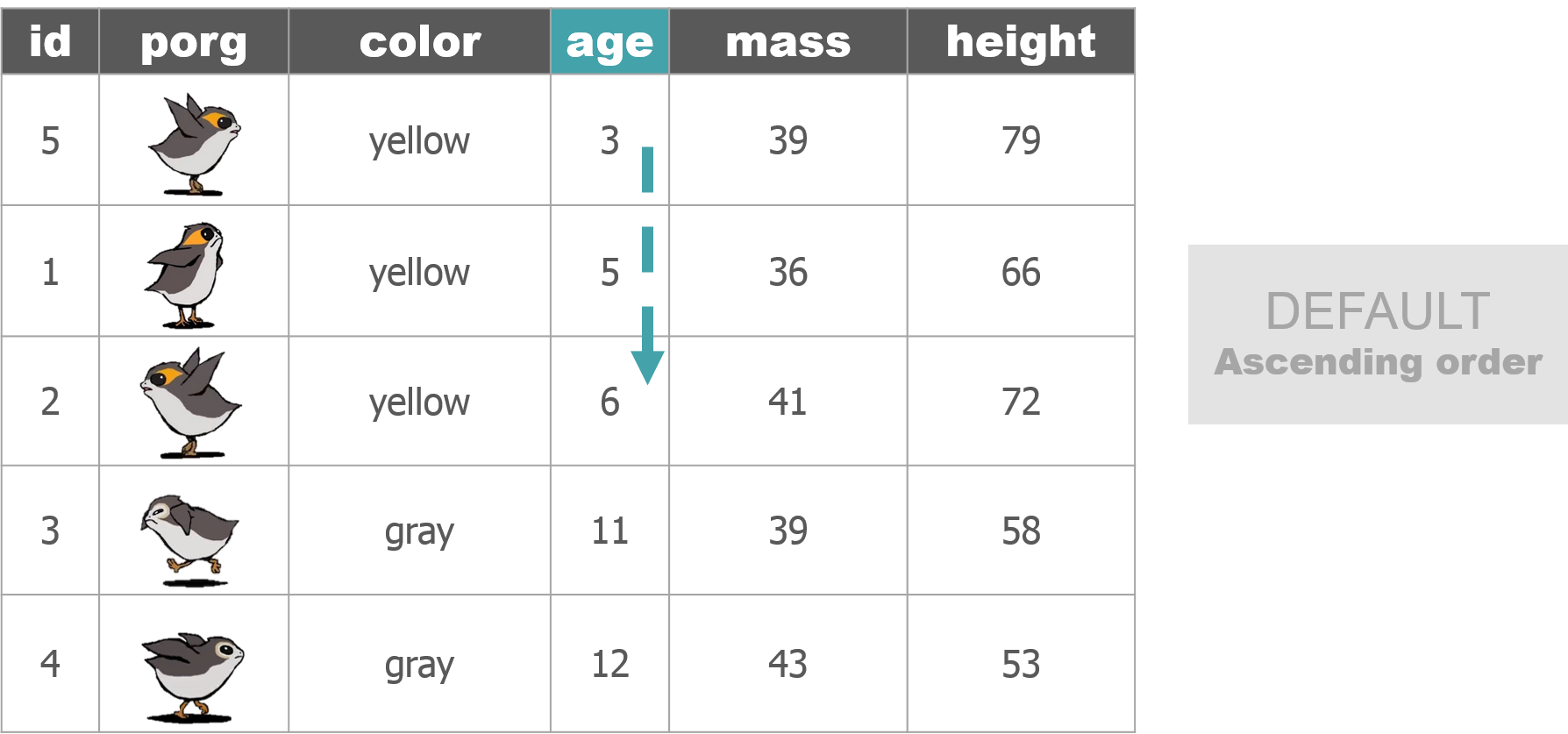
## # ... with 1,122 more rows6 | arrange()
Rey wants to know what the highest priced items are. Use arrange() to find the highest priced scrap item and see which origins might have a lot of them.
# Arrange scrap items by price
scrap <- arrange(scrap, price_per_pound)

# View the top 6 rows
head(scrap)
## # A tibble: 6 x 7
## receipt_date item origin destination amount units price_per_pound
## <chr> <chr> <chr> <chr> <dbl> <chr> <dbl>
## 1 4/4/2013 Aural se~ Tuanul Raiders 707 Tons 145.
## 2 5/22/2013 Aural se~ Outskirts Niima Outp~ 3005 Tons 145.
## 3 5/23/2013 Aural se~ Tuanul Raiders 6204 Tons 145.
## 4 6/4/2013 Aural se~ Tuanul Raiders 3120 Tons 145.
## 5 6/10/2013 Aural se~ Blowback~ Niima Outp~ 2312 Tons 145.
## 6 6/20/2013 Aural se~ Outskirts Trade cara~ 6272 Tons 145.Only 145 credits! That’s not very much at all, oh wait…
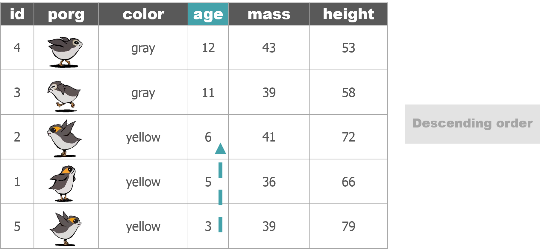
Put BIG things first: desc()
To arrange a column in descending order with the biggest numbers on top, we use: desc(price_per_pound)
# Put most expensive items on top
scrap <- arrange(scrap, desc(price_per_pound))

# View the top 8 rows
head(scrap, 8)
## # A tibble: 8 x 7
## receipt_date item origin destination amount units price_per_pound
## <chr> <chr> <chr> <chr> <dbl> <chr> <dbl>
## 1 12/31/2016 Total All All 2.97e6 Tons 579215.
## 2 4/10/2013 Sublight~ Outskirts Niima Outp~ 1.06e4 Tons 7211.
## 3 4/14/2013 Sublight~ Outskirts Raiders 2.38e3 Tons 7211.
## 4 4/15/2013 Sublight~ Craterto~ Raiders 6.31e3 Tons 7211.
## 5 4/16/2013 Sublight~ Tuanul Trade cara~ 3.98e3 Tons 7211.
## 6 5/14/2013 Sublight~ Craterto~ Raiders 2.99e2 Tons 7211.
## 7 6/14/2013 Sublight~ Blowback~ Raiders 8.58e3 Tons 7211.
## 8 8/6/2013 Sublight~ Craterto~ Raiders 1.77e3 Tons 7211.Exercise
Try arranging by more than one column, such as price_per_pound and amount. What happens?
HINT: You can view the entire table by clicking on it in the upper-right Environment tab.
Pro-tip!
When you save an arranged data table it maintains its order. This is perfect for sending people a quick Top 10 list of pollutants or sites.
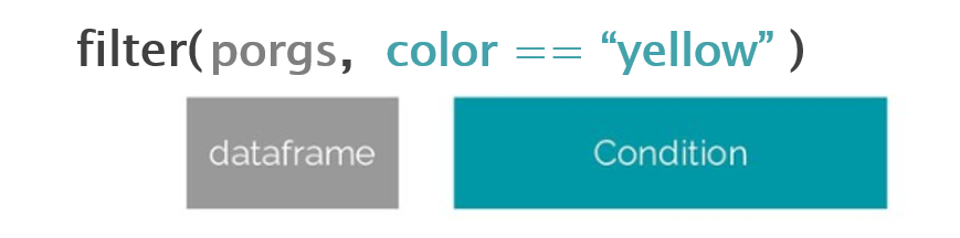
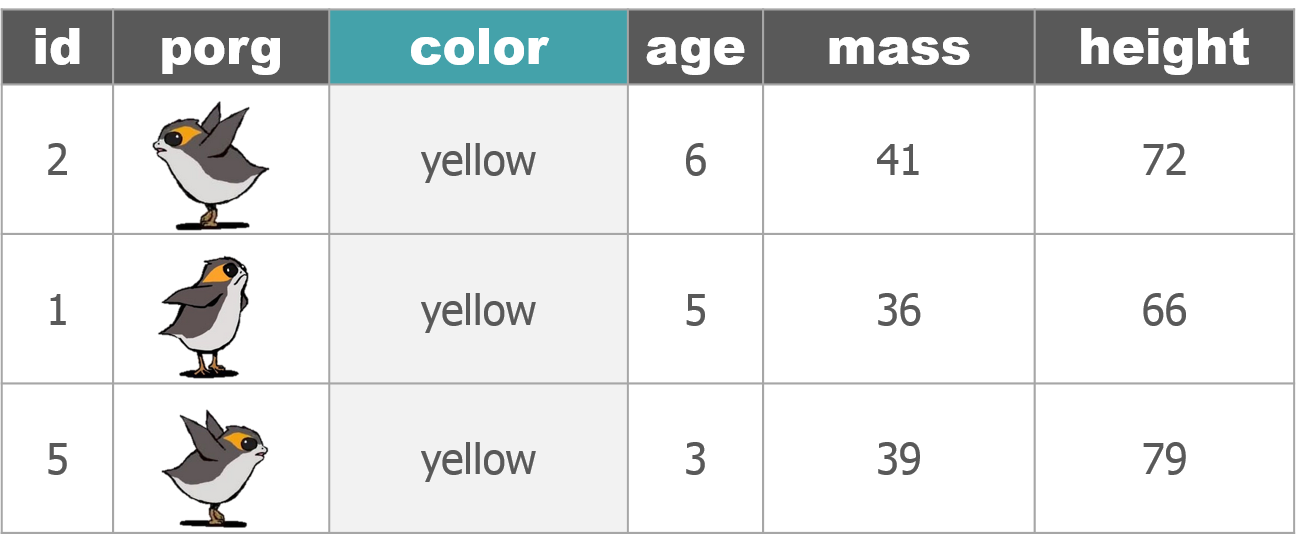
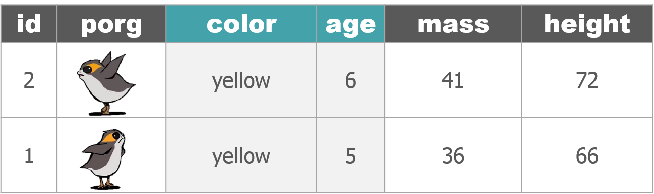
7 | filter()
The filter() function creates a subset of the data based on the value of one or more columns. Let’s take a look at the records with the origin "All".
filter(scrap, origin == "All")## # A tibble: 1 x 7
## receipt_date item origin destination amount units price_per_pound
## <chr> <chr> <chr> <chr> <dbl> <chr> <dbl>
## 1 12/31/2016 Total All All 2971601 Tons 579215.Pro-tip!
Use a == (double equals sign) for comparing values. A == makes the comparison “is it equal to?” and returns a True or False answer. So the code above returns all the rows where the condition origin == "All" is TRUE.
A single equals sign = is used within functions to set options, for example read_csv(file = "starwars_scrap_jakku.csv"). Don’t worry too much. If you use the wrong symbol R is often helpful and will let you know which one is needed.
Comparisons
Processing data requires many types of filtering. You’ll want to know how to select observations in your table by making various comparisons.
Key comparison operators
| Symbol | Comparison |
|---|---|
> |
greater than |
>= |
greater than or equal to |
< |
less than |
<= |
less than or equal to |
== |
equal to |
!= |
NOT equal to |
%in% |
is value in a list: X %in% c(1,3,5) |
is.na(...) |
Is the value missing? |
Exercise
Try comparing some things in the console and see if you get what you’d expect. R doesn’t always think like we do.
4 != 5

4 == 4

4 < 3

4 > c(1, 3, 5)

5 == c(1, 3, 5)

5 %in% c(1, 3, 5)

2 %in% c(1, 3, 5)

2 == NA
Dropping rows
Let’s look at the data without that pesky All category. Look in the comparison table above to find the NOT operator. We’re going to filter the data to keep only the origins that are NOT equal to “All”.
scrap <- filter(scrap, origin != "All")We can arrange the data in ascending order by item to confirm that the “All” category is gone.
# Arrange data
scrap <- arrange(scrap, item)

head(scrap)
## # A tibble: 6 x 7
## receipt_date item origin destination amount units price_per_pound
## <chr> <chr> <chr> <chr> <dbl> <chr> <dbl>
## 1 4/4/2013 Aural se~ Tuanul Raiders 707 Tons 145.
## 2 5/22/2013 Aural se~ Outskirts Niima Outp~ 3005 Tons 145.
## 3 5/23/2013 Aural se~ Tuanul Raiders 6204 Tons 145.
## 4 6/4/2013 Aural se~ Tuanul Raiders 3120 Tons 145.
## 5 6/10/2013 Aural se~ Blowback~ Niima Outp~ 2312 Tons 145.
## 6 6/20/2013 Aural se~ Outskirts Trade cara~ 6272 Tons 145.Now let’s take another look at that bar chart. Is there anything else that is less than perfect with our data?
library(ggplot2)

ggplot(scrap, aes(x = origin, y = amount)) + geom_col()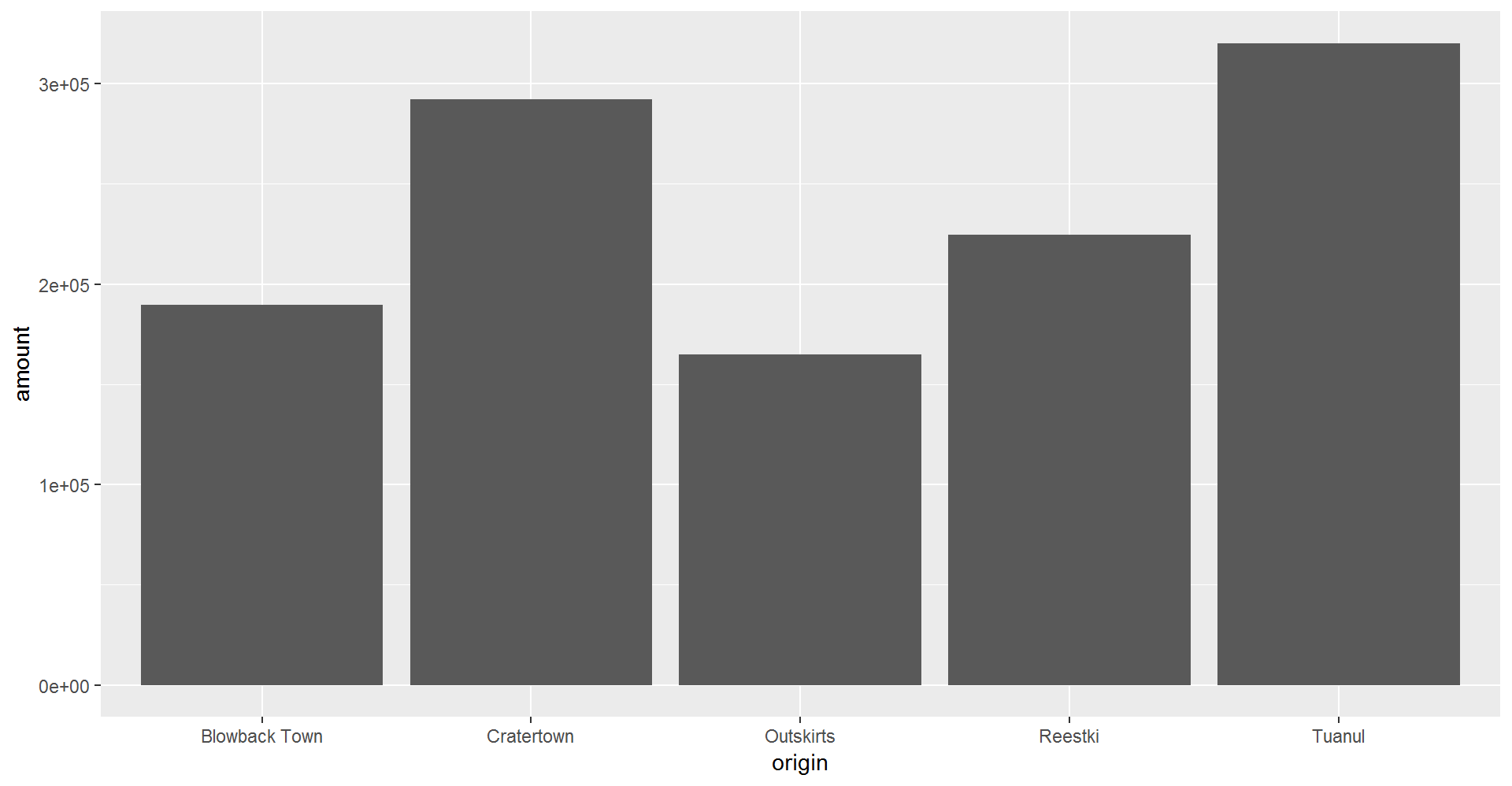
Multiple filters
We can add multiple comparisons to filter() to further restrict the data we pull from a larger data set. Only the records that pass the conditions of all the comparisons will be pulled into the new data frame.
The code below filters the data to only scrap records with an origin of Outskirts AND a destination of Niima Outpost.
outskirts_to_niima <- filter(scrap,
                             origin        == "Outskirts",
                             destination   == "Niima Outpost")
Guess Who?
Star Wars edition

Are you the best Jedi detective out there? Let’s play a game and find out.
Guess what else comes with the dplyr package? A Star Wars data set.
You can open the data set with the following steps:
- Load the
dplyrpackage from yourlibrary() - Pull the Star Wars dataset into your environment.
library(dplyr)

starwars_data <- starwars
Rules
- You have a secret identity.
- Scroll through the Star Wars dataset and find a character you find interesting. (Or run
sample_n(starwars_data, 1)to choose your character at random.) - Keep it hidden! Don’t show your neighbor the character you chose.
- Take turns asking each other questions about your partner’s Star Wars character.
- Use the answers to build a
filter()function and narrow down the potential characters your neighbor may have picked.
For example: Here’s a filter() statement that filters the data to the character Plo Koon.
mr_koon <- filter(starwars_data,
                  mass       < 100,
                  eye_color  != "blue",
                  gender     == "male",
                  homeworld  == "Dorin",
                  birth_year > 20)
Elusive answers are allowed. For example, if someone asks: What is your character’s mass?
- You can respond: My character’s mass is equal to one less than their age.
- Or if you’re feeling generous you can give a straight forward answer such as: My character’s mass is definitely more than 100 and less that 140.
Sometimes a character will not have a specific attribute. We learned earlier how R stores nulls as NA. If your character has a missing value for hair color, one of your filter statements could be is.na(hair_color).
WINNER!
The winner is the first to guess their neighbor’s character.
WINNERS Click here!
Want to rematch?
How about make it best of 3 games?
Back to Jakku
Let’s calculate some new columns to help focus Rey’s scavenging work.
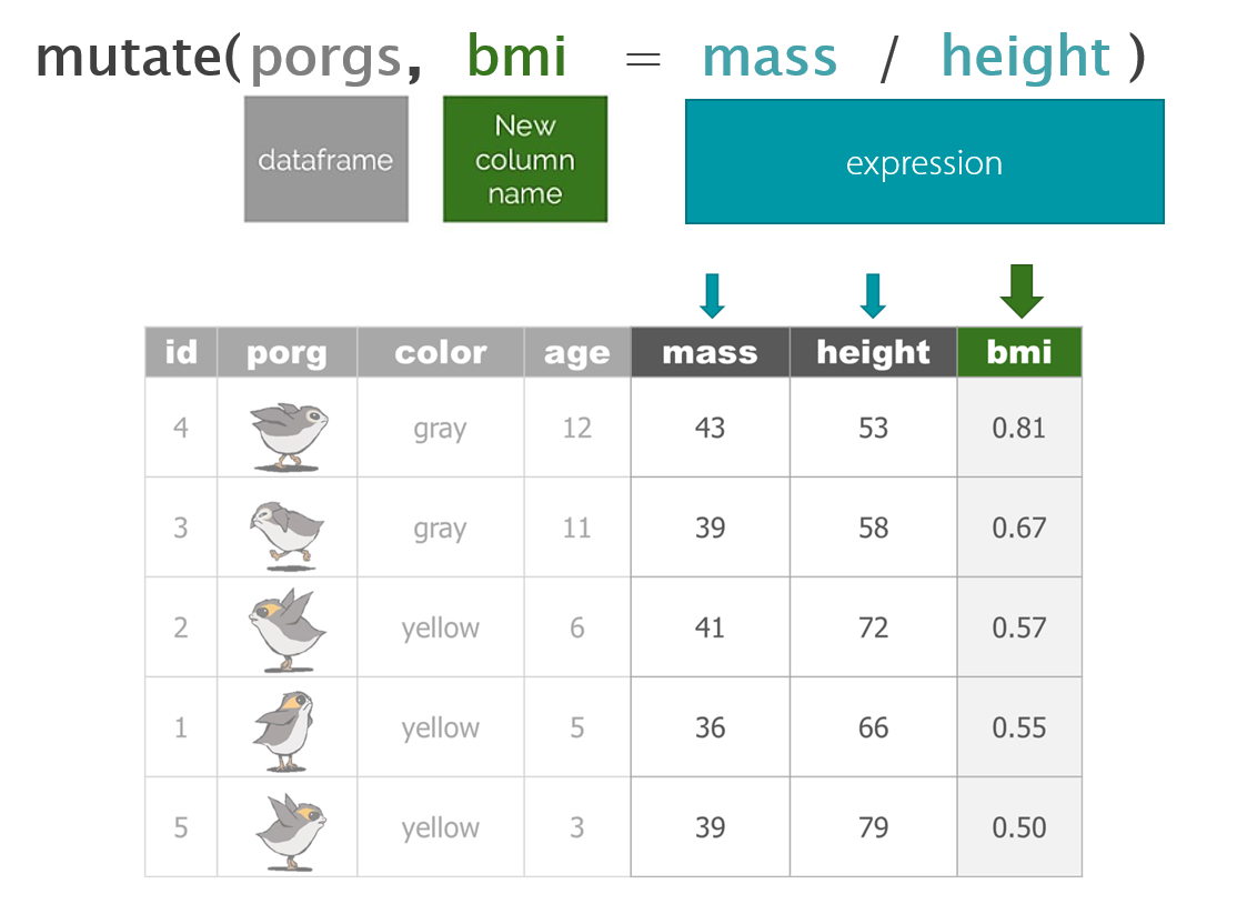
8 | mutate()
mutate() can edit existing columns in a data frame or add new values that are calculated from existing columns.
Add a column
First, let’s add a column with our names. That way Rey can thank us personally when her ship is finally up and running.
# Add your name as a column
scrap <- mutate(scrap, scrap_finder = "BB8")
Add several columns
Let’s also add a new column to document the data measurement method.
#  Add your name as a column and
#  some information about the method
scrap <- mutate(scrap,
                scrap_finder    = "BB8",
                measure_method  = "REM-24")

## REM = Republic Equivalent Method
Change a column
Remember how the units of Tons was written two ways: “TONS” and “Tons”? We can use mutate() together with tolower() to make sure all of the scrap units are written in lower case. This will help prevent them from getting grouped separately in our plots and summaries.
# Set units to all lower-case
scrap <- mutate(scrap, units = tolower(units))

# toupper() changes all of the letters to upper-case.
Add calculated columns
In our work we often use mutate to convert units for measurements. In this case, let’s estimate the total pounds for the scrap items that are reported in tons.
Tons to Pounds conversion
We can use mutate() to convert the amount column to pounds. Multiply the amount column by 2000 to get new values for a column named amount_lbs.
scrap_pounds <- mutate(scrap, amount_lbs = amount * 2000)Final stretch!
We now have all the tools we need. To get her ship working, Rey is trying to track down more of the scrap item: Ion engine.
Step 1:
- filter the data to only
Ion engine
Show code
# Grab only the items named "Ion engine"
scrap_pounds <- filter(scrap_pounds, item == "Ion engine")
Now, arrange the data in descending order of pounds so Rey knows where the highest amount of Ion engine scrap comes from.
Step 2:
- arrange in descending order by
amount_lbs
Show code
# Arrange data
scrap_pounds <- arrange(scrap_pounds, desc(amount_lbs))

# Return the origin of the highest amount_lbs of scrap
head(scrap_pounds, 1)

# Plot the total amount_lbs by origin
ggplot(scrap_pounds, aes(x = origin, y = amount_lbs)) +
  geom_col()
Pop Quiz!
For the item Ion engine, which origin has the highest amount_lbs?
Tuanul
Cratertown
Outskirts
Reestki
Show solution
Cratertown
Yes!! You receive the ship parts to repair Rey’s Millennium Falcon. Onward!
First mission complete!
Nice work!
Rey got a great deal on her engines and even traded in some scrap for spending cash.
Time to get off this dusty planet, we’re flying to Endor!

9 | Save data
You can’t break your original dataset if you always name it something else. Let’s use the readr package to save our new CSV with the tons converted to pounds.
# Save data as a CSV file
write_csv(scrap_pounds, "scrap_in_pounds.csv")
Where did R save the file?
Let’s create a new results/ folder to keep our processed data separate from any raw data we receive.
# Save data as a CSV file to results folder
write_csv(scrap_pounds, "results/scrap_in_pounds.csv")
New mission available
BB8 received new data from the wookies suggesting there was a large magnetic storm just before Site 1 burned down on Endor. Sounds like we’re going to be STORM CHASERS tomorrow. Mission accepted.