R Training | Day 1
Welcome!
The force is strong with you. Join us, learn R, and use your powers for good.
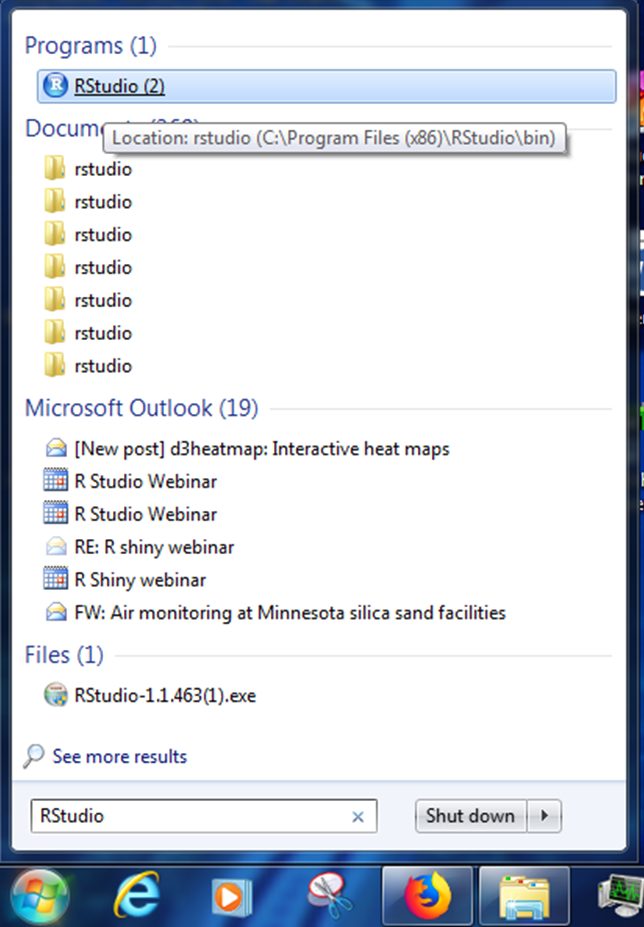
Power on your droids

You and BB8 arrived just in time. Rey needs your help!
The Junk boss Unkar is up to no-good once again and Rey needs some parts to repair her starship. With your help she can escape Jakku and join forces with the New Republic.
Connect to your droid
- Open the Start menu (the Windows logo on the bottom left of the screen)
- Select
Remote Desktop Connection(you may need to search for it the 1st time) - Enter your desktop’s ID:
w7-your7digit#orR32-your7digit# - Press Connect
Open RStudio
Where’s my R? Do you need to install R or RStudio? There’s a nice workaround for you below.
Get R! (workaround)
This is a temporary solution to get R + RStudio on your computer for the training.
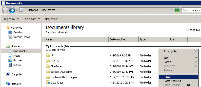
1. Open the R versions folder on the X-drive
\\pca.state.mn.us\xdrive\Agency_Files\Data_Services\DAU\Data Analytics User Group\Shared\r\versions
2. Select and copy these 2 folders
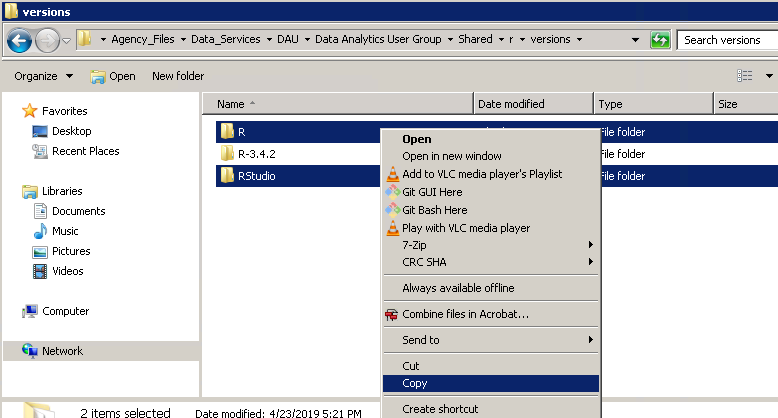
3. Open your Documents folder
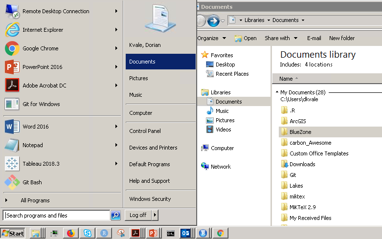
4. Paste in the copied folders
Test for success
- Open
RStudio.exein theRStudio\binfolder
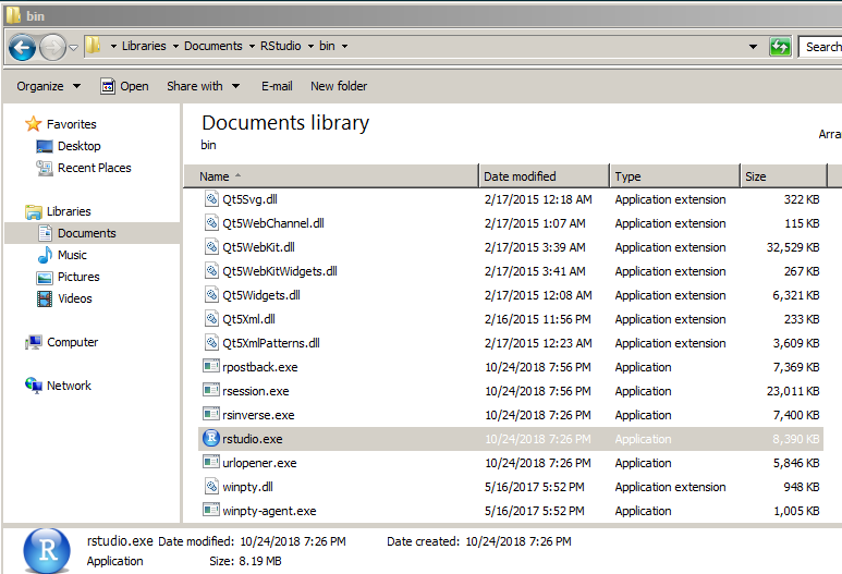
- If you see the screen below - Great work! You’re ready to go.

Still no R? No worries. You can use R online at RStudio Cloud.
Introductions

Let’s introduce ourselves and the data we love. Find a partner and get to know 3 things about them.
Things to share
- Your name or Star Wars alias
- Types of data you have
- Who you share it with
- What you want to get from the workshop
- The messiest & funniest part of your data
- Something you get to do over and over again
Hint: Maybe this is something you can automate with R
What’s my name?


We are Barbara, Kristie, Dorian, and Derek. Yes, we look exactly like our profile photos above.
We aren’t computer scientists and that’s okay!
We make lots of mistakes. Mistakes are funny. You can laugh with us.
Why R?
R Community
- See the R Community page.
- MPCA sharing + questions - R questions
- Finding R Help - Get Help!
- R cheatsheets
When do we use R?
- To connect to databases
- To read data from websites
- To document and share methods
- When data will have frequent updates
- When we want to improve a process over time
R is for reading
Lucky for us, programming doesn’t have to be a bunch of math equations. R allows you to write your data analysis in a step-by-step fashion, much like creating a recipe for cookies. And just like a recipe, we can start at the top and read our way down to the bottom.
Blast off!
1 | RStudio - The grand tour
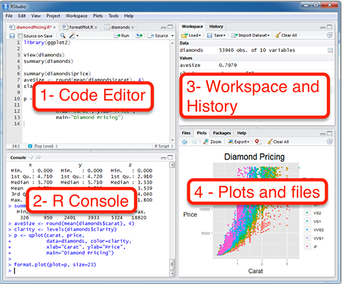
1 - Code Editor
This is where you write your scripts and document your work. The tabs at the top of the code editor allow you to view scripts and data sets you have open. This is where you’ll spend most of your time.
2 - R Console
This is where code is actually executed by the computer. It shows code that you have run and any errors, warnings, or other messages resulting from that code. You can input code directly into the console and run it, but it won’t be saved for later. That’s why we like to run all of our code directly from a script in the code editor.
3 - Workspace
This pane shows all of the objects and functions that you have created, as well as a history of the code you have run during your current session. The environment tab shows all of your objects and functions. The history tab shows the code you have run. Note the broom icon below the Connections tab. This cleans shop and allows you to clear all of the objects in your workspace.
4 - Plots and files
These tabs allow you to view and open files in your current directory, view plots and other visual objects like maps, view your installed packages and their functions, and access the help window. If at anytime you’re unsure what a function does, enter it’s name after a question mark. For example, try entering ?mean into the console and push ENTER.
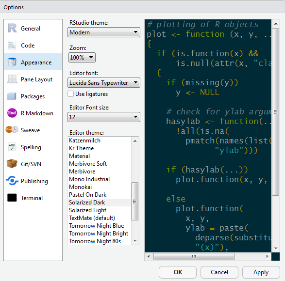
Customize R Studio
Make it your own
Let’s add a little style so R Studio feels like home. Follow these steps to change the font-size and and color scheme:
- Go to Tools on the top navigation bar.
- Choose
Global Options... - Choose
Appearancewith the paint bucket. - Increase the
Editor Font size - Pick an Editor theme you like.
- We’ll be using
Dreamweaverfor the class
- We’ll be using
Now that we’re ready, let’s go forth and make some trouble. While BB8 works on tracking down some data for us from his droid friends, we’ll get to know our way around his internal computer.
Data awaits us…

Start an R project
Let’s make a new project for our Jakku mischief.
Step 1: Start a new project
- In Rstudio select File from the top menu bar
- Choose New Project…
- Choose New Directory
- Choose New Project
- Enter a project name such as
"starwars" - Select Browse… and choose a folder where you normally perform your work.
- Click Create Project
Step 2: Open a new script
- File > New File > R Script
- Click the floppy disk save icon
- Give it a name:
jakku.Rorlesson1.Rwill work well
2 | Names and things
You can assign values to new objects using the “left arrow” <-, which is written by typing a less-than sign followed by a hyphen. It’s more officially known as the assignment operator. Try adding the code below to your R script to assign a value to an object called droid.
To run a line of code in your script, move the cursor to that line and press CTRL+ENTER.
Assignment operator
# Create a new object
droid <- "bb8"

droid

wookie <- "Chewbacca"

wookie
Break some things
# To save text to a character object you need quotation marks: "text"

# Try this:
wookie <- Chewbacca
## Error in eval(expr, envir, enclos): object 'Chewbacca' not foundERROR
Without quotes, R looks for an object called Chewbacca, and then lets you know that it couldn’t find one.
Copy objects
# To copy an object, assign it to a new name
wookie2 <- wookie


# Or overwrite an object with new "text"
wookie <- "Tarfful"

wookie


# Did this change the value stored in wookie2?
wookie2
Drop and remove data
You can drop objects with the remove function rm(). Try it out on some of your wookies.
# Delete objects to clean-up your environment
rm(wookie)

rm(wookie2)
Exercise!
How can we get the ‘wookie’ object back?
HINT: The UP arrow in the Console is your friend.
EXPLORE: Deleting data is okay
Don’t worry about deleting data or objects in R. You can always recreate them! When R loads data files it copies the contents and cuts off any connection to the original data. So your original data files remain safe and won’t suffer any accidental changes. That means if something disappears or goes wrong in R, it’s okay. We can always reload the data using our script.
What’s a good name?
Everything has a name in R and you can name things almost anything you like. You can even name your data TOP_SECRET_shhhhhh... or Luke_I_am_your_father or data_McData_face.
Sadly, there are a few minor restrictions. Names cannot include spaces or special characters that might be found in math equations, like +, -, *, \, /, =, !, or ).
Exercise!
Try running some of these examples. Find new ways to create errors. The more broken the better! Half of learning R is finding what doesn’t work.
n wookies <- 5

n*wookies <- 5

n_wookies <- 5

n.wookies <- 5


all_the_wookies! <- "Everyone on Kashyyyk"
# You can add one wookie
n_wookies <- n_wookies + 1
# But what if you have 10,000 wookies?
n_wookies <- 10,000
# They also cannot begin with a number.
1st_wookie <- "Chewbacca"
88b <- "droid"
# But they can contain numbers!
wookie1 <- "Chewbacca"
bb8 <- "droid"EXPLORE: What happens when we re-created n_wookies the 2nd time?
When we create a new object with the same name as something that already exists, the new object replaces the old one. Sometimes we want to update an existing object and replace the old version. Other times we may want to copy an object to a new name to preserve the original.
This is similar to choosing between
SaveandSave Aswhen saving a file.
Multiple items
We can add multiple values inside c() to make a vector of items. It’s like a chain of items, where each additional item is connected by a comma. The c stands for to concatenate or to combine values into a vector.
Let’s use c() to create a few vectors of names.
# Create a character vector and name it starwars_characters
starwars_characters <- c("Luke", "Leia", "Han Solo")

# Print starwars_characters to the console
starwars_characters
## [1] "Luke" "Leia" "Han Solo"# Create a numeric vector and name it starwars_ages
starwars_ages <- c(19,19,25)
# Print the ages to the console
starwars_ages## [1] 19 19 25Make a table
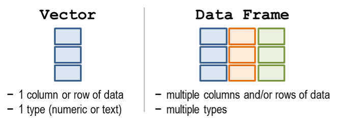
A table in R is known as a data frame. We can think of it as a group of columns, where each column is made from a vector. Data frames in R have columns of data that are all the same length.
Let’s make a table with 2 columns to hold the character names and their ages.
# Create table with columns "character" and "ages" with values from the starwars_names and starwars_ages vectors
starwars_df <- data.frame(character = starwars_characters,
                          ages  = starwars_ages)

# Print the starwars_df data frame to the console
starwars_df
## character ages
## 1 Luke 19
## 2 Leia 19
## 3 Han Solo 25Exercise
Create the same table above, but add a 3rd column that lists their father names:
c("Darth", "Darth", "Unknown")
starwars_df <- data.frame(character   = starwars_characters,
                          ages        = starwars_ages,
                          fathers     = __________________)
starwars_df <- data.frame(character   = starwars_characters,
                          ages        = starwars_ages,
                          fathers     = c("Darth", "Darth", "Unknown"))
Show all values in a $column_name
Use the $ sign after the name of your table to see the values in one of your columns.
# View the "ages" column in starwars_df
starwars_df$ages
## [1] 19 19 25Pop Quiz, hotshot!
Which of these object names are valid? (Hint: You can test them.)
my starwars fandom
my_wookies55
5wookies
my-wookie
Wookies!!!
Show solution
my_wookies55
Yes!! The FORCE is strong with you!
Leave a #comment
The lines of code in the scripts that start with a # in front are called comments. Every line that starts with a # is ignored and won’t be run as R code. You can use the # to add notes in your script to make it easier for others and yourself to understand what is happening and why. You can also use comments to add warnings or instructions for others using your code.
3 | Read data
The first step of a good scrap audit is reading in some data to figure out where all the scrap is coming from. Here is a small dataset showing the scrap economy on Jakku. It was salvaged from a crash site, but the transfer was incomplete.
| origin | destination | item | amount | price_d |
|---|---|---|---|---|
| Outskirts | Raiders | Bulkhead | 332 | 300 |
| Niima Outpost | Trade caravan | Hull panels | 1120 | 286 |
| Cratertown | Plutt | Hyperdrives | 45 | 45 |
| Tro—- | Ta—- | So—* | 1 | 10—- |
This looks like it could be useful. Now, if only we had some more data to work with…
New Message (1)
Incoming… BB8
BB8: Beep boop Beep.
BB8: I intercepted a large scrapper data set from droid 4P-L of Junk Boss Plutt.
Receiving data now…
scrap_records.csv
item,origin,destination,amount,units,price_per_pound
Flight recorder,Outskirts,Niima Outpost,887,Tons,590.93
Proximity sensor,Outskirts,Raiders,7081,Tons,1229.03
Aural sensor,Tuanul,Raiders,707,Tons,145.27
Electromagnetic filter,Tuanul,Niima Outpost,107,Tons,188.2
...
You: Yikes! This looks like a mess! What can I do with this?
CSV to the rescue
The main data format used in R is the CSV (comma-separated values). A CSV is a simple text file that can be opened in R and most other stats software, including Excel. It looks squished together as plain text, but that’s okay! When opened in R, the text becomes a familiar looking table with columns and rows.
Before we launch ahead, let’s add a package to R that will help us read CSV files.
How to save a CSV from Excel
Step 1: Open your Excel file.
Step 2: Save as CSV
- Go to File
- Save As
- Browse to your project folder
- Save as type: _CSV (Comma Delimited) (*.csv)_
- Any of the CSV options will work
- Any of the CSV options will work
- Click Yes
- Close Excel (Click “Don’t Save” as much as you need to. Seriously, we just saved it. Why won’t Excel just leave us alone?)
Return to RStudio and open your project. Look at your Files tab in the lower right window. Click on the CSV file you saved and choose View File. Success!
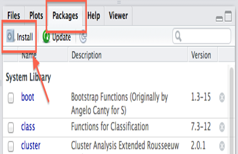
📦 Add new packages
What is an R package?
A package is a small add-on for R, it’s like a phone App for your phone. They add capabilities like statistical functions, mapping powers, and special charts to R. In order to use a new package we first need to install it. Let’s try it!

The readr package helps import data into R in different formats. It helps you out by cleaning the data of extra white space and formatting tricky date formats automatically.
Add a package to your library
- Open RStudio
- Type
install.packages("readr")in the lower left console - Press Enter
- Wait two seconds
- Open the
Packagestab in the lower right window of RStudio to see the packages in your library- Use the search bar to find the
readrpackage
- Use the search bar to find the
Your installed packages are stored in your R library. The Packages tab on the right shows all of the available packages installed in your library. When you want to use one of them, you load it in R. Loading a package is like opening an App on your phone. To load a package we use the library() function. Once you load it, the package will stay loaded until you close RStudio.
Let’s load the readr package so we can use the read_csv() function to read the Jakku scrap data.
Read the data
library(readr)

read_csv("https://itep-r.netlify.com/data/starwars_scrap_jakku.csv")
## Parsed with column specification:
## cols(
## receipt_date = col_character(),
## item = col_character(),
## origin = col_character(),
## destination = col_character(),
## amount = col_double(),
## units = col_character(),
## price_per_pound = col_double()
## )## # A tibble: 1,132 x 7
## receipt_date item origin destination amount units price_per_pound
## <chr> <chr> <chr> <chr> <dbl> <chr> <dbl>
## 1 4/1/2013 Flight re~ Outski~ Niima Outp~ 887 Tons 591.
## 2 4/2/2013 Proximity~ Outski~ Raiders 7081 Tons 1229.
## 3 4/3/2013 Vitus-Ser~ Reestki Raiders 4901 Tons 226.
## 4 4/4/2013 Aural sen~ Tuanul Raiders 707 Tons 145.
## 5 4/5/2013 Electroma~ Tuanul Niima Outp~ 107 Tons 188.
## 6 4/6/2013 Proximity~ Tuanul Trade cara~ 32109 Tons 1229.
## 7 4/7/2013 Hyperdriv~ Tuanul Trade cara~ 862 Tons 1485.
## 8 4/8/2013 Landing j~ Reestki Niima Outp~ 13944 Tons 1497.
## 9 4/9/2013 Electroma~ Crater~ Raiders 7788 Tons 188.
## 10 4/10/2013 Sublight ~ Outski~ Niima Outp~ 10642 Tons 7211.
## # ... with 1,122 more rowsName the data
Where did the data go after you read it into R? When we want to work with the data in R, we need to give it a name with the assignment operator: <-.
# Read in scrap data and set name to "scrap"
scrap <- read_csv("https://itep-r.netlify.com/data/starwars_scrap_jakku.csv")

# Type the name of the table to view it in the console
scrap
## # A tibble: 1,132 x 7
## receipt_date item origin destination amount units price_per_pound
## <chr> <chr> <chr> <chr> <dbl> <chr> <dbl>
## 1 4/1/2013 Flight re~ Outski~ Niima Outp~ 887 Tons 591.
## 2 4/2/2013 Proximity~ Outski~ Raiders 7081 Tons 1229.
## 3 4/3/2013 Vitus-Ser~ Reestki Raiders 4901 Tons 226.
## 4 4/4/2013 Aural sen~ Tuanul Raiders 707 Tons 145.
## 5 4/5/2013 Electroma~ Tuanul Niima Outp~ 107 Tons 188.
## 6 4/6/2013 Proximity~ Tuanul Trade cara~ 32109 Tons 1229.
## 7 4/7/2013 Hyperdriv~ Tuanul Trade cara~ 862 Tons 1485.
## 8 4/8/2013 Landing j~ Reestki Niima Outp~ 13944 Tons 1497.
## 9 4/9/2013 Electroma~ Crater~ Raiders 7788 Tons 188.
## 10 4/10/2013 Sublight ~ Outski~ Niima Outp~ 10642 Tons 7211.
## # ... with 1,122 more rowsPro-tip!
Notice the row of <three> letter abbreviations under the column names? These describe the data type of each column.
<chr>stands for character vector or a string of characters. Examples: “apple”, “apple5”, “5 red apples”
<int>stands for integer. Examples: 5, 34, 1071
<dbl>stands for double. Examples: 5.0000, 3.4E-6, 10.7106
We’ll discover more data types later on, such as dates and logical (TRUE/FALSE).
Pop Quiz!
1. What data type is the destination column?
letters
character
TRUE/FALSE
numbers
Show solution
character
Woop! You got this.
2. What package does read_csv() come from?
dinosaur
get_data
readr
dplyr
Show solution
readr
Great job! You are Jedi worthy!
3. How would you load the package junkfinder?
junkfinder()
library(junkfinder)
load(junkfinder)
gogo_gadget(junkfinder)
Show solution
library("junkfinder")
Excellent! Keep the streak going.
EXPLORE: Change a function’s options
Functions often have options that you can change to control their behavior. You can set these optins using arguments. Let’s look at a few of the arguments for the function read_csv().
Skip a row
Sometimes you may want to ignore the first row in your data file, especially an EPA file that includes a disclaimer on the first row. Yes EPA, we’re looking at you. Please stop.
Let’s open the help window with ?read_csv and try to find an argument that can help us. There’s a lot of them! But the skip argument looks like it could be helpful. Take a look at the description near the bottom. The default is skip = 0, which reads every line, but we can skip the first line by writing skip = 1. Let’s give it a go.
read_csv("https://itep-r.netlify.com/data/starwars_scrap_jakku.csv", skip = 1)Limit the total number of rows
Other types of data have weird last rows that are a subtotal or just report “END OF DATA”. Sometimes we want read_csv to ignore the last row, or only pull in a million lines because you don’t want to bog down the memory on an old laptop.
Let’s look through the help window to find an argument that can help us. Type ?read_csv and scroll down.
The n_max argument looks like it could be helpful. The default is n_max = Inf, which means it will read every line, but we can limit the lines we read to only one hundred by using n_max = 100.
# Read in 100 rows
small_data <- read_csv("https://itep-r.netlify.com/data/starwars_scrap_jakku.csv", skip = 1, n_max = 100)

# Remove the data
rm(small_data)
Show me the arguments!
To see all of a function’s arguments
- Enter its name in the console followed by a parenthesis:
read_csv( | - Press
TABon the keyboard - This brings up a drop-down menu of the available arguments for that function
4 | ggplot2
Plot the data, Plot the data, Plot the data

In data analysis it is really important to look at your data early and often. For that, let’s add a new package called ggplot2!
Install it by running the following in your Console:
install.packages("ggplot2")
NOTE
You can also install packages from the Packages tab in the lower right window of RStudio.
A column plot
Here’s a simple chart showing the total amount of scrap for each origin location.
library(ggplot2)## Warning: package 'ggplot2' was built under R version 3.5.3ggplot(scrap, aes(y = amount, x = origin)) +
geom_col() +
theme_gray()## Warning: Removed 910 rows containing missing values (position_stack).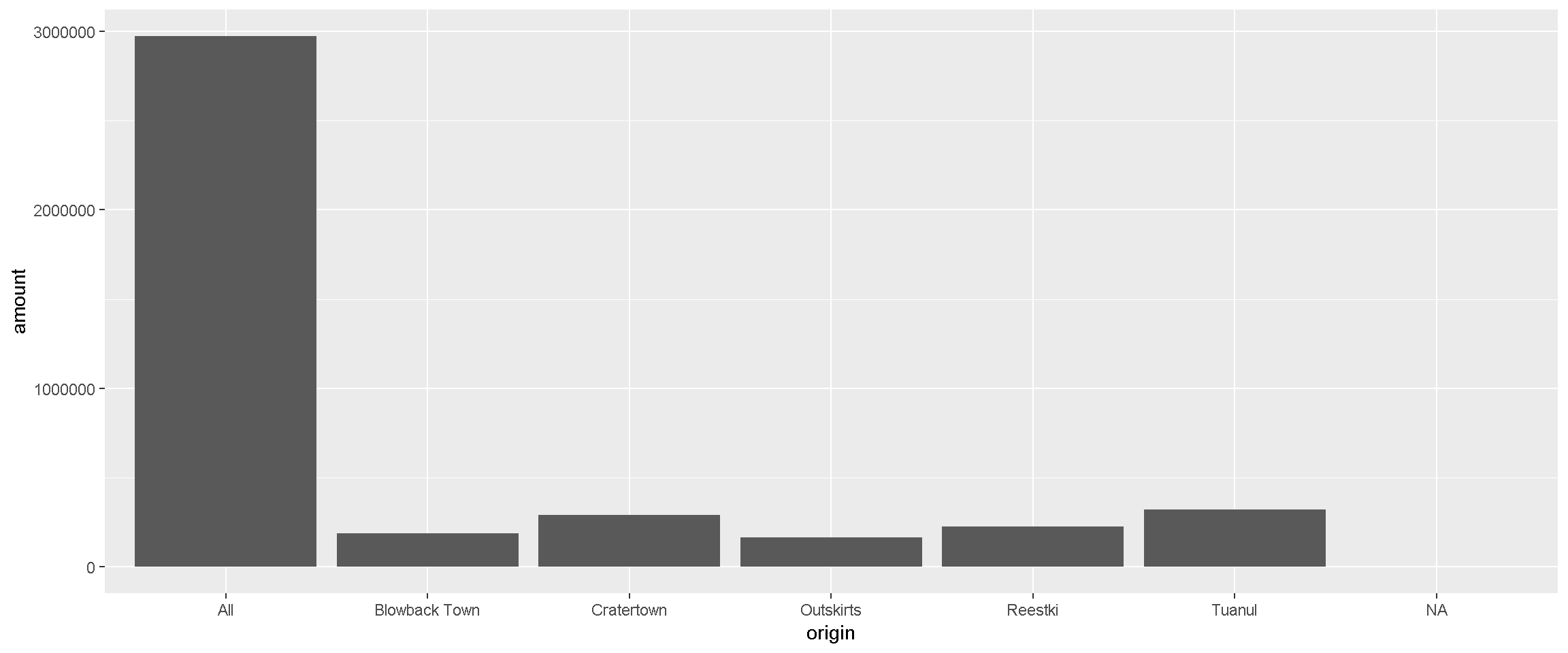
Well, well, well, it looks like there is an All category we should look into more. Either there is a town hogging all the scrap or the data needs some cleaning.
Exercise
Try changing theme_gray() to theme_dark(). What changes on the chart? What stays the same?
Try another theme: theme_classic() or theme_void() or delete the entire line and the + above to see what the default settings are.
You can view all of the available theme options at ggplot2 themes.
5 | Get help
Lost in an ERROR message? Is something behaving strangely and want to know why? See the Help! page for some troubleshooting options.
6 | Operation Shut Down
When you close R for the first time you will see some options about saving your workspace and other files. In general, we advise against saving these files. It’s easy enough to re-run your script next time you open your project. This will help RStudio open a fresh and clean environment every time you start it.
Follow these steps to set these options permanently.
Turn off Save Workspace
- Go to
Tools > Global Options....on the top RStudio navigation bar - On the first screen:
RECAP
What packages have we added to our
library?What new functions have we learned?
REVIEW: Functions & arguments
Functions perform steps based on inputs called arguments and usually return an output object. There are functions in R that are really complex but most boil down to the same general setup:
new_output <- function(argument_input1, argument_input2)You can make your own functions in R and name them almost anything you like, even my_amazing_starwars_function().

You can think of a function like a plan for making Clone Troopers.
create_clones(host       = "Jango Fett",
              n_troopers = 2000)
The function above creates Clone Troopers based on two arguments: the host and n_troopers. When we have more than one argument, we use a comma to separate them. With some luck, the function will successfully return a new object - a group of 2,000 Clone Troopers.
The sum() function
We can use the sum() function to find the sum age of our Star Wars characters.
# Call the sum function with starwars_ages as input
ages_sum <- sum(starwars_ages) # Assigns the output to starwars_ages_sum

# Print the starwars_ages_sum value to the console
ages_sum
## [1] 63The sum() function takes the starwars_ages vector as input, performs a calculation, and returns a number. Note that we assigned the output to the name ages_sum.
If we don’t assign the output it will be printed to the console and not saved.
# Alternative without assigning output
sum(starwars_ages)
## [1] 63NOTE
The original
starwars_agesvector has not changed. Each function has its own “environment” and its calculations happen inside a bubble. In general, what happens inside a function won’t change your objects outside of the function.
starwars_ages## [1] 19 19 25 EXPLORE: Does the order of arguments matter?
You may be wondering why we included skip = for the skip argument, but tell R explicitly what argument the other objects belonged to. Well now, that’s an interesting story. When you pass inputs to a function, R assumes you’ve entered them in the same order that is shown on the ?help page. Let’s say you had a function called feed_porgs() with 3 arguments:
feed_porgs(breakfast = "fish", lunch = "veggies", dinner = "clams").
A shorthand to write this would be:
feed_porgs("fish", "veggies", "clams").
This works out just fine because all of the arguments were entered in the default order, the same as above.
But let’s say we write:
feed_porgs("veggies", "clams", "fish")
Now the function will send veggies to the porgs for breakfast because that is the first argument. But that’s no good for the porgs. So if we really want to write “veggies” first, we’ll need to tell R which food item belongs to which meal.
Like this:
feed_porgs(lunch = "veggies", breakfast = "fish", dinner = "clams").
Ok, so what about read_csv()?
For read_csv, when we wrote:
read_csv(scrap_file, column_names, skip = 1)
R assumes that the first argument (the data file) is scrap_file and that the 2nd argument “col_names” should be set to column_names. Next, the skip = argument is included explicitly because skip is the 10th argument in read_csv(). If we didn’t include skip =, R would assume the value 1 that we entered is meant for the function’s 3rd argument.
Key terms
package |
An add-on for R that contains new functions that someone created to help you. It’s like an App for R. | |
library |
The name of the folder that stores all your packages, and the function used to load a package. | |
function |
Functions perform an operation on your data and returns a result. The function sum() takes a series of values and returns the sum for you. |
|
argument |
Arguments are options or inputs that you pass to a function to change how it behaves. The argument skip = 1 tells the read_csv() function to ignore the first row when reading in a data file. To see the default values for a function you can type ?read_csv in the console. |
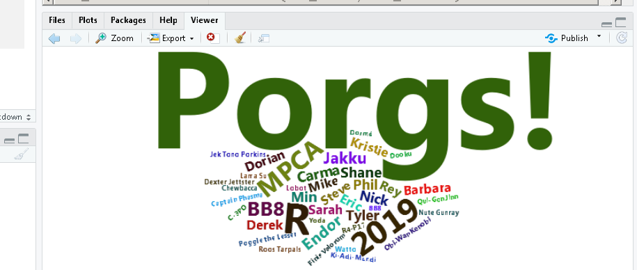
BONUS Build your own Word Cloud
Let’s launch ourselves into the unknown and use R to make a Word Cloud. With a little copy-pasting we can make a fun image out of everyone’s name in the class.
Since you’re such a big deal, we can also help you make your name really BIG .
INSTRUCTIONS
Open R Studio
Copy the code below into your script in RStudio. Start with the line
install.packagesand end with the linecolor = 'random-dark').
install.packages(c("wordcloud2", "dplyr"))
library(wordcloud2)
library(dplyr)

           #---- Class names ----#
class <- c("Steve"    = 8,
           "Mike"     = 9,
           "Eric"     = 8,
           "Hannah"   = 9,
           "Jon"      = 8,
           "Mary"     = 9,
           "Min"      = 9,
           "Aida"     = 9,
           "Matthias" = 8,
           "Gao"      = 9,
           "Ben"      = 9,
           "Eva"      = 9,
           "James"    = 10,
           "Kitty"    = 11,
           "Zeb"      = 9,
           #---- Fun names ----#
           "R"        = 26,
           "2019"     = 20,
           "MPCA"     = 16,
           "Porgs!"    = 84,
           "Endor"     = 10,
           "Jakku"     = 10,
           "BB8"       = 12,
           "Rey"       = 8,
           "Derek"     = 8,
           "Kristie"   = 8,
           "Barbara"   = 8,
           "Dorian"    = 8)

# Add 20 Star Wars names as small text, size = 4
class <- c(class, rep(4, 20))

names(class)[(length(class) - 19):length(class)] <- sample_n(starwars, 20)$name

# Plot the Word Cloud with the "random-dark" color theme
wordcloud2(data.frame(word = names(class), freq = class),
           size  = 1,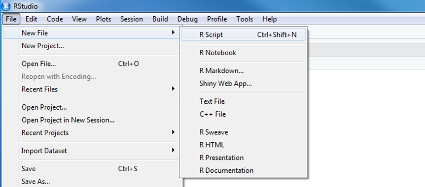
color = 'random-dark')- In R Studio click on File > New File > R Script. You will see a code editor window open.
- Paste the copied code into the upper left hand window. This is your code editor.
- Highlight all of the code and hit
CTRL + ENTER. - You should see a Word Cloud pop up in the lower right of RStudio.
- Now try increasing the number next to your name.
- Run the code again.
- You may need to increase the size of the
Viewerwindow shown below to make enough room for your name to appear. You can also click theZoomicon to create a bigger word cloud.
- You may need to increase the size of the
- Make your name even BIGGER!